Category Archives: Antennas

A Ferrite Rod Loop for NDB DX: Generation 3

Resonant Loops (RLs) are an often overlooked form of receiving antenna, but remain my favorite, both from a performance viewpoint and also from a viewpoint of passion: I love the things! Although they are not by any means as popular as their remote cousins, the Shielded Magnetic Loop (SML), RLs can in some environments offer performance which an SML simply cannot match. With careful design and construction, RLs can exhibit a very high loaded Q which can give the loop:

1) A very high degree of frequency selectivity right in the antenna, often to the point where additional front end filtering is not necessary to protect the receiver from spurious responses. Case in point: in my area, there are a number of 50 kW MW stations, and to use my Wellbrook SML for NDB DXing, I MUST use a 9th order lowpass filter. Such a filter is not needed when DXing NDBs with a Ferrite Rod RL.

2) A very low Minimum Discernible Signal; RLs can have a sensitivity which belies their size.

3) RLs tend to be amplified loops, but a high Q in the antenna can drastically reduce the gain requirements of the following amplifier.

4) A well balanced RL will generally exhibit strong directionality. In some loops at some frequencies, an RL can discriminate reception based on the arrival azimuth. Peaks and nulls may be observed. At the very least, an RL can discriminate against local noise, and I have observed noise depression of up to 30 dB when I have had an RL mounted on a rotator.

5) An RL tends to be small, and can generally be sited in a quiet area on one’s lot to keep it away from power or utility lines, houses, etc.

As well as their advantages, RLs as a receiving antenna have a number of disadvantages.

1) Without band switching (and this is not always feasible), RLs have a finite tuning range (Fmax over Fmin), and this is generally within the range of 3:1 to 5:1. This tends to make an RL an “Application Specific” antenna.

2) The lack of commercial offerings means that you are most likely going to have to roll your own; RLs tend to be a construction project by the user.

3) There are countless gripes on the internet by users who dislike the fact that they must be re-tuned constantly as the receiver frequency is changed. They have missed the point by a country mile; the magic in a RL is in its narrowband nature and mo’ narrow mo’ better. Generally.

4) Although physically small (we are talking about small receiving loops here), to fully realize the sensitivity which a small RL can offer, the RL MUST be sited outdoors. This complicates the tuning of the loop, as the capacitance used to tune the loop MUST be located physically close to the loop winding. Using varactors to tune a loop remotely is pretty easy, but if the target Q of the loop requires the use of a mechanical variable capacitor (as this LF Ferrite Loop does), then it becomes a substantially more complicated process to tune the loop remotely.

5) RLs are generally considered to be unshielded and thus prone to signal corruption from local RFI. This is not true, and most resonant loops can be built with an effectice electrostatic shield.

Over the past winter and spring, I have been working on a prototype of a Ferrite Rod RL which would be suitable for DXing LF NDBs. Some of the progress and logs have been posted here:

http://www.hfunderground.com/board/index.php/topic,19471.0.html

http://www.hfunderground.com/board/index.php/topic,19868.0.html

http://www.hfunderground.com/board/index.php/topic,20896.0.html

I have been extremely encouraged by the performance of the prototypes, and have been working on a “Generation 3″ version of the loop which should be deployed by this fall. I cannot do much about the first 2 “disadvantages” listed above, but the G3 loop and its control system are being designed to attack problems 3 and 4 head on, and offer some functionality which will greatly aid in the DXing of LF NDBs. Some of the key points are:

1) Design of a Stepping Motor Gear Train which will allow precise tuning of a mechanical variable capacitor located out near the loop site (about 160 ft away). In the current design, there are approximately 4800 motor steps per full 180 degree traverse of the tuning capacitor, which is just about the minimum required for the loaded Q of this Ferrite Rod RL.

2) Utilization of an Arduino SBC in the loop head. The Arduino firmware implements a Server (a simple command interpreter) which will control the Geared Stepping Motor used in the gear train via a standard off the shelf Stepper Shield for the Arduino. It will also allow control of additional loop parameters from within the shack.

3) The system will be controlled (tuned) via a Client application which will run on the same computer as the SDR control app (at this point I am using SDR Console V 1.5). At this point, RC is coded against a small subset of the SDR Console CAT Command vocabulary, but more is possible in the future.

n.b. There have been a large number of design decisions to make in this project. The choice of the SDR control program to code against (at least initially) was kinda critical. I have 2 favorites: SdrDx and SDR Console, and I have been able to programmatically control both via apps I have written. As good as SdrDx is (and it is very very good), I prefer using the older version of SDR Console (the version with the infinite license) for NDB DXing. Its ability to present full screen views of the waterfall and spectrum without control clutter is a huge aid in DXing, and its ability to simultaneously display a Zoom window with a span of 2 or 5 kHz really aids in fine tuning a loop. Additionally, I really love the palette control in SDR Console; quick very fine adjustments in the palette allow the app to function as its own QRSS viewer, and the ability to visually DX piled up NDBs really lessens the fatigue you encounter when trying to hear a particular NDB in a pileup. The fact that communication with SDR Console is easy via a free Virtual Serial Port Manager (such as VSPE) is a big plus.

4) The Client app (at this point boringly named Remote Controller or RC) will encapsulate a number of functional blocks in individual Tab Pages in a TabControl in the following categories:

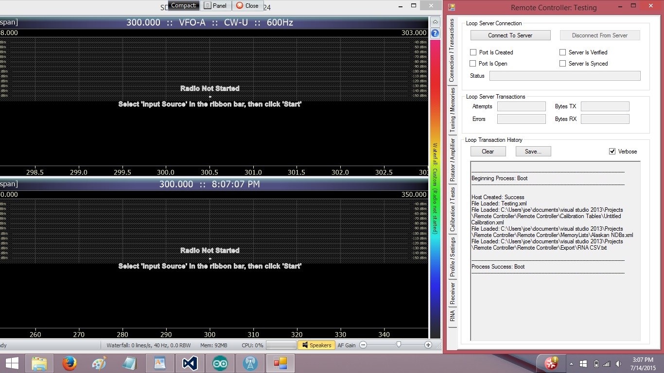
A) Server Connection/Transactions: This page contains the controls to open, maintain, and handle a network connection to the Loop Server out in the yard.

B) Tuning/Memory Lists: RC will implement a set of tuning controls, some of which are programmable, to accomplish Loop and Receiver tuning. RC will enable the user to create Memory Lists which are displayed in a ListView Control, and which can act as a tuning source by double clicking an item in the list. I consider this to be a very powerful feature which might help in DXing NDBs this fall. I imagine loading in a general list of NDBs at the start of a session to gauge what cards the Great Gods of Propagation has dealt out. From these “prop beacon beacons”, I might determine, for example, that commonly heard stations in Nunavut are in well, and I could then prepare (­­or load in a previously prepared) Memory List of Nunavutian NDBs to see if I can hear anything new without having to navigate through the online RNA list.

C) Station Database: In NDB DXing, I find the RNA NDB list to be absolutely indispensable. RC has the ability to import a prepared copy of the RNA Excel download file, and this list is displayed in toto on a tab page in RC. RC displays the list in a CheckedListView Control. Double-clicking an item will execute it (tune the Loop and also the Receiver to the NDB frequency). Individually selected items can be checked and exported to a Memory List. The list is searchable (by call with wildcards, by ITU country, by State/Province, etc.). Search results can be exported to a Memory List. This means that it is a very simple process to generate a custom Memory List for all NDBs in Alaska, for example.

D) Receiver: RC can open and maintain a connection via a Virtual Serial Port to the SDR Console app running on the same Windows box. Tuning the loop can simultaneously tune the SDR to the RL resonant frequency (right now the accuracy is about +/- 2 kHz), but fine tuning of the loop is easy. In fact, in NDB DXing, the RL is more often than not tuned to one of the sideband frequencies, and not the carrier referenced in frequency lists.

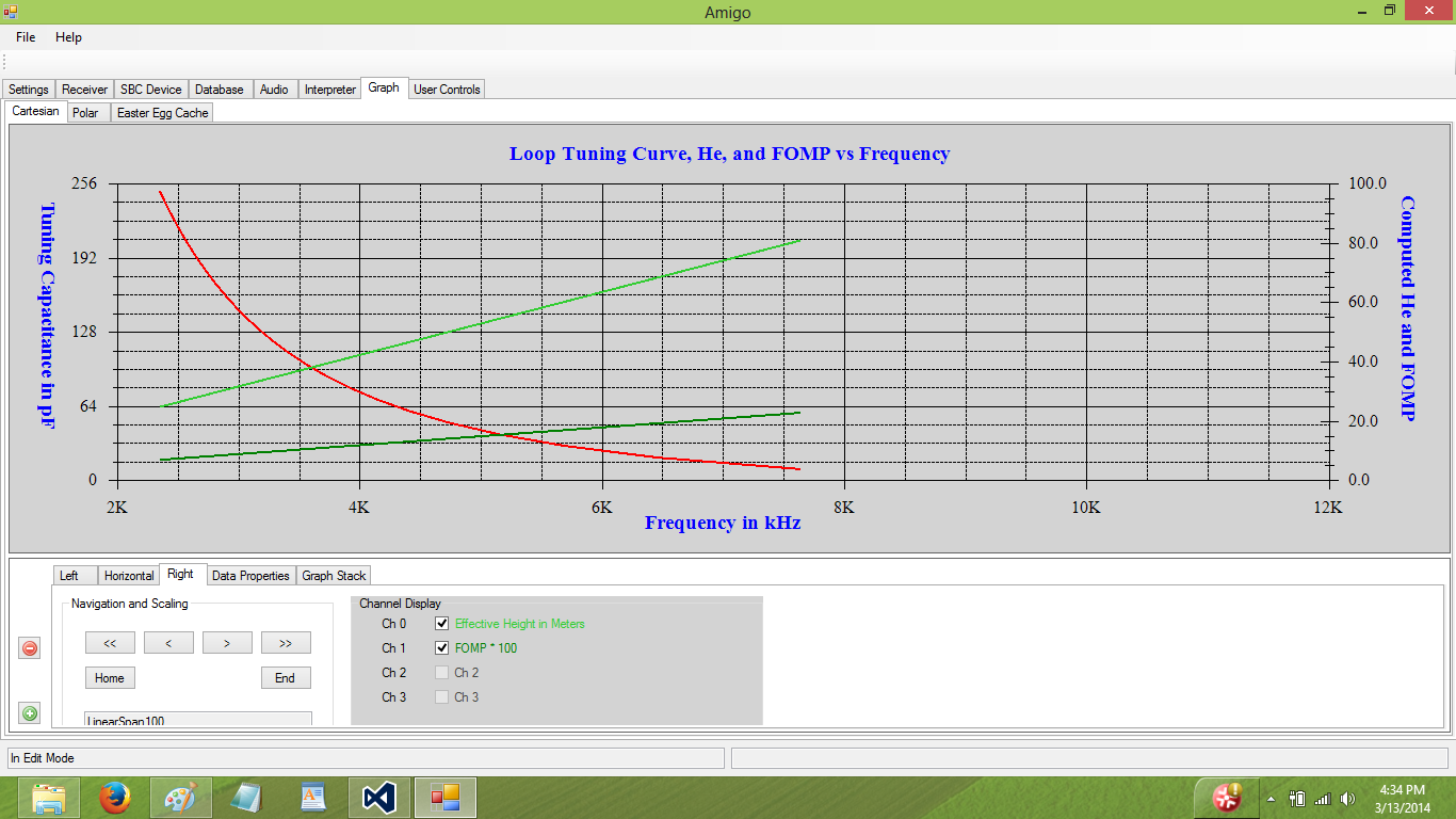
E) Calibration/Testing: Since a calibration curve of the antenna response (motor steps versus resonant frequency) is required, RC contains Antenna Calibration functionality which allows a semi-automated approach to antenna calibration. Calibration Curve data can be viewed graphically. RC also implements a number of built-in test suites which can be used to test the loop, receiver, and rotator performance, and can help the app to function as a tool for further development.

F) Rotator/Amplifier: Since RNA logs also contain a Maidenhead Locator field, from this Longitude and Latitude can be easily computed; this allows further computation of both Bearing to the NDB and also Range. I am adding control of a modified Antenna Rotator to the client app RC so that selecting an item in either a Memory or RNA list would (with one double-click) tune the Loop, tune the SDR, and rotate the Loop to the proper Azimuth. Rotation can then be manually controlled once it is at the proper az.

G) Profile/Settings: RC supports a Profile file, and uses it to store settings between sessions. The user can generate a profile which can be used to control various types of loops.

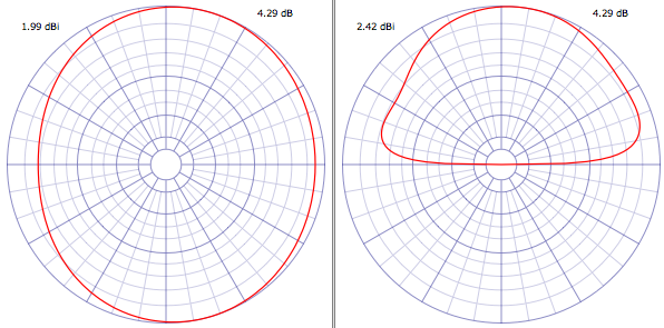
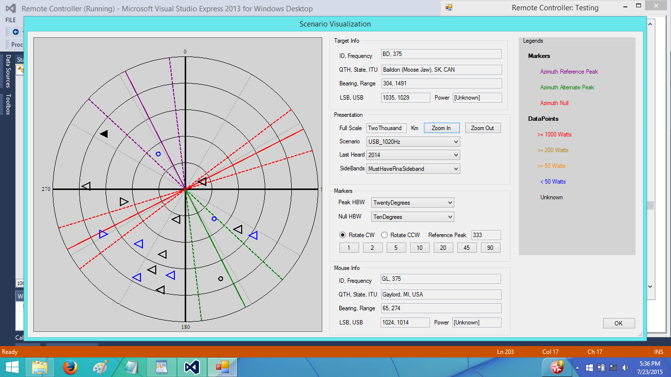
H) Normally, a Memory List item will contain all RNA fields, and when double clicked, the antenna and SDR will be tuned, and the rotator will be spun to the azimuth which can be computed from the RNA Maidenhead locator field. This azimuth will be the bearing of peak rod reception, but more often than not, this will not be the desired antenna bearing; one would in theory like to rotate the antenna to the bearing which will possibly give the best reception considering all of the co-channel NDBs which would interfere with the desired NDB. The loop generally has a broad reception peak and a narrow null (or depression) minima, and we would like to have these in the proper orientation with respect to co-channel interference.

RC incorporates a Scenario Visualization tool. Right clicking an item in the RNA list will open the Visualization dialog. This will present a polar plot of Bearing vs Range on which all potentially interfering NDBs will be plotted, as well as the target NDB. The plot will also render markers representing the Peak and Null beams of the antenna, and these will be rendered with variable width beam widths. The antenna patterns can be rotated with respect to the plotted NDBs, and the user can select a best guess antenna rotation for the target NDB. This target RNA entry can then be exported to a Memory List, and any time the item is double clicked in the Memory List, the rotator will be rotated to the preferred (and not the Maidenhead) azimuth. This will enable me to create Memory List of highly desired high value targets, and will allow me to efficiently check these targets in any DX session.

A Block Diagram of the system is:

Block Diagram

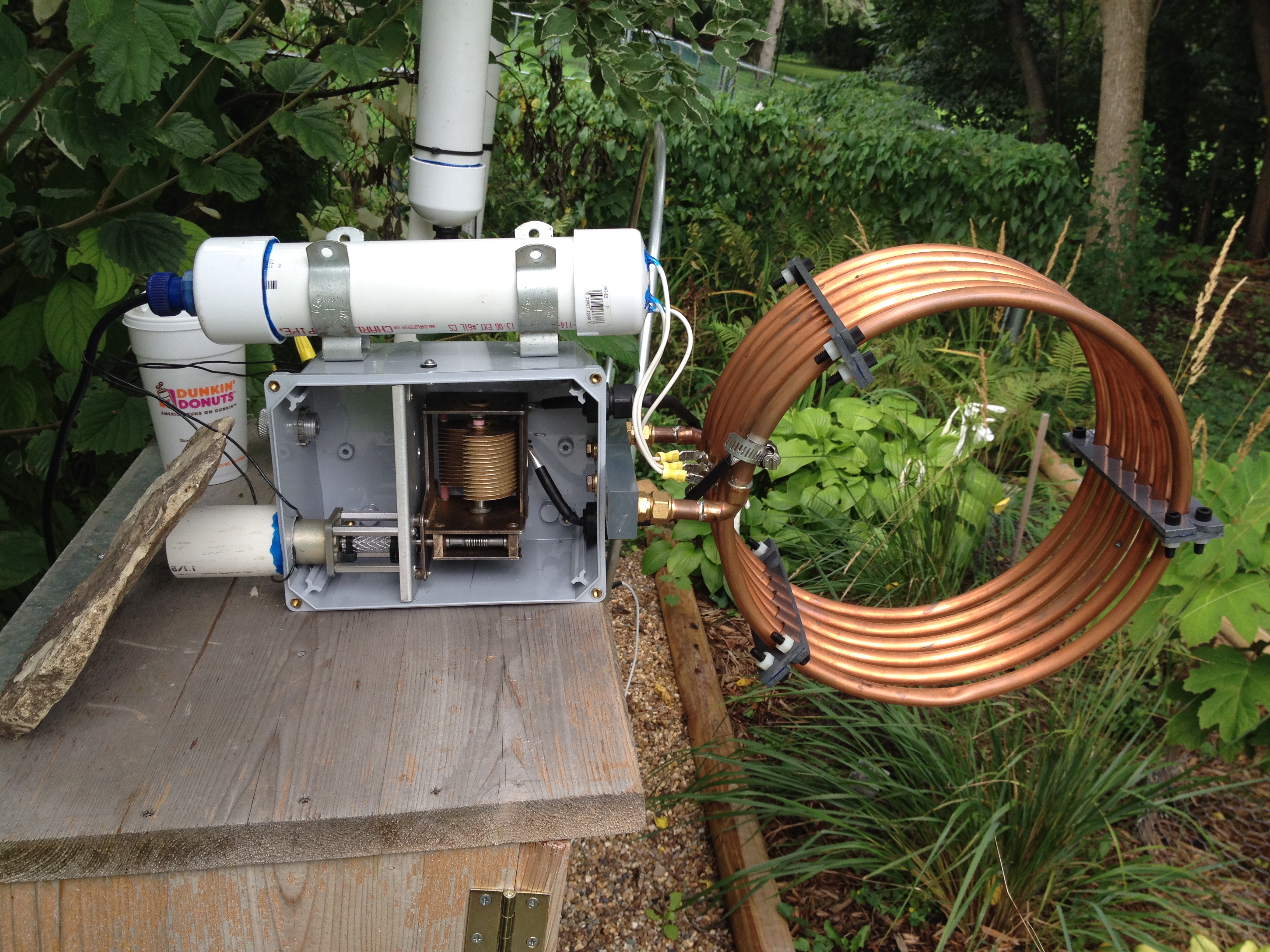
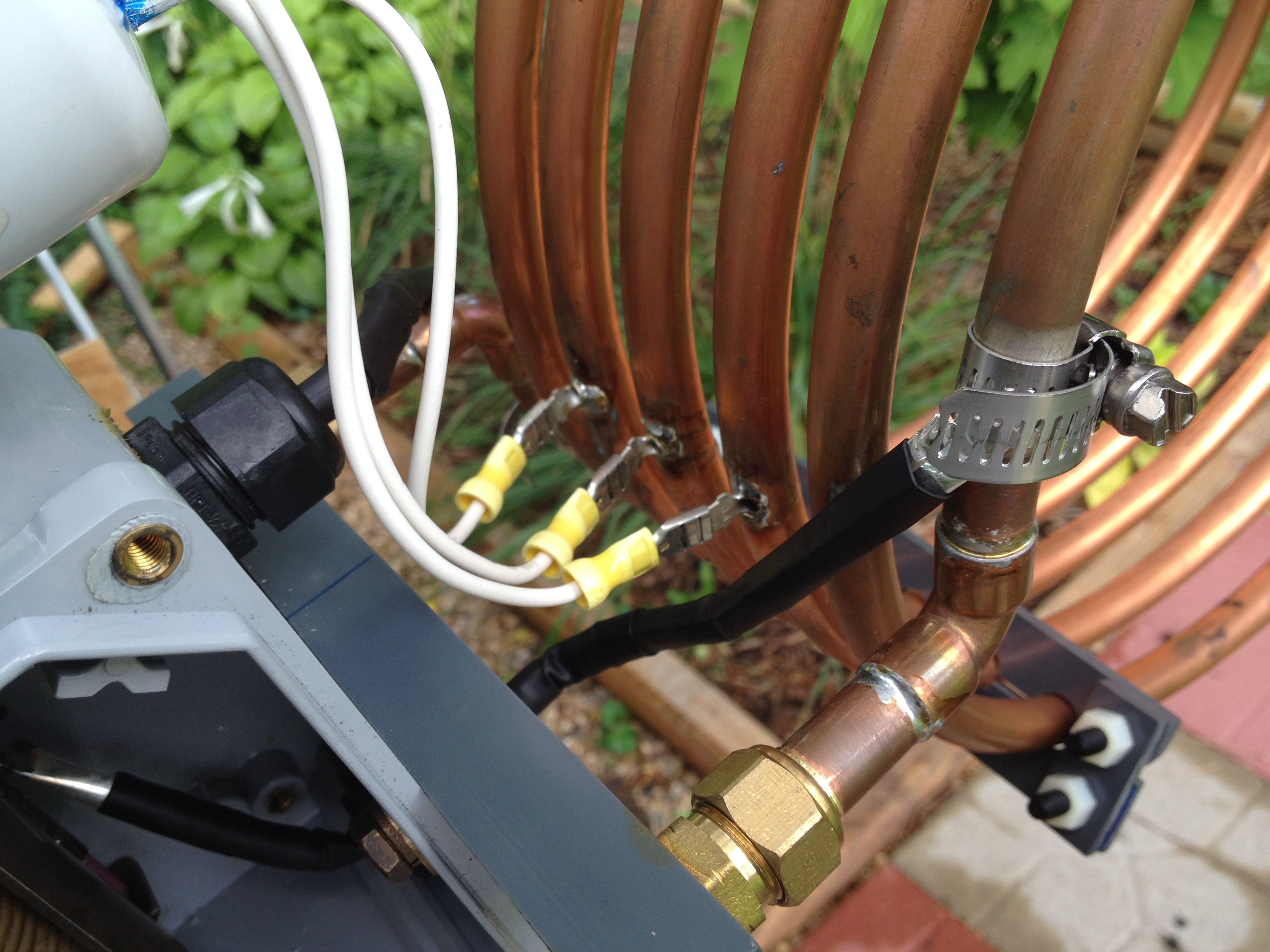
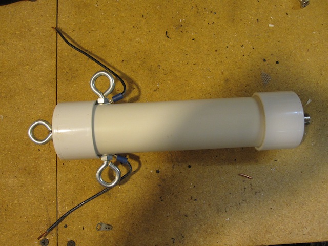
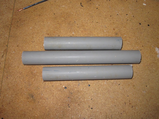
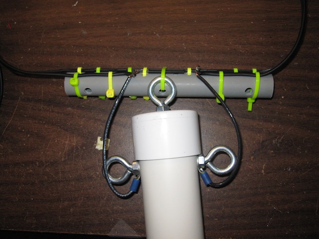
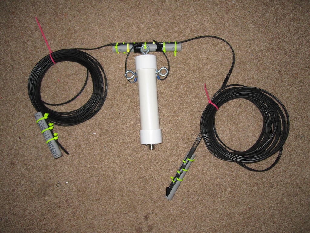
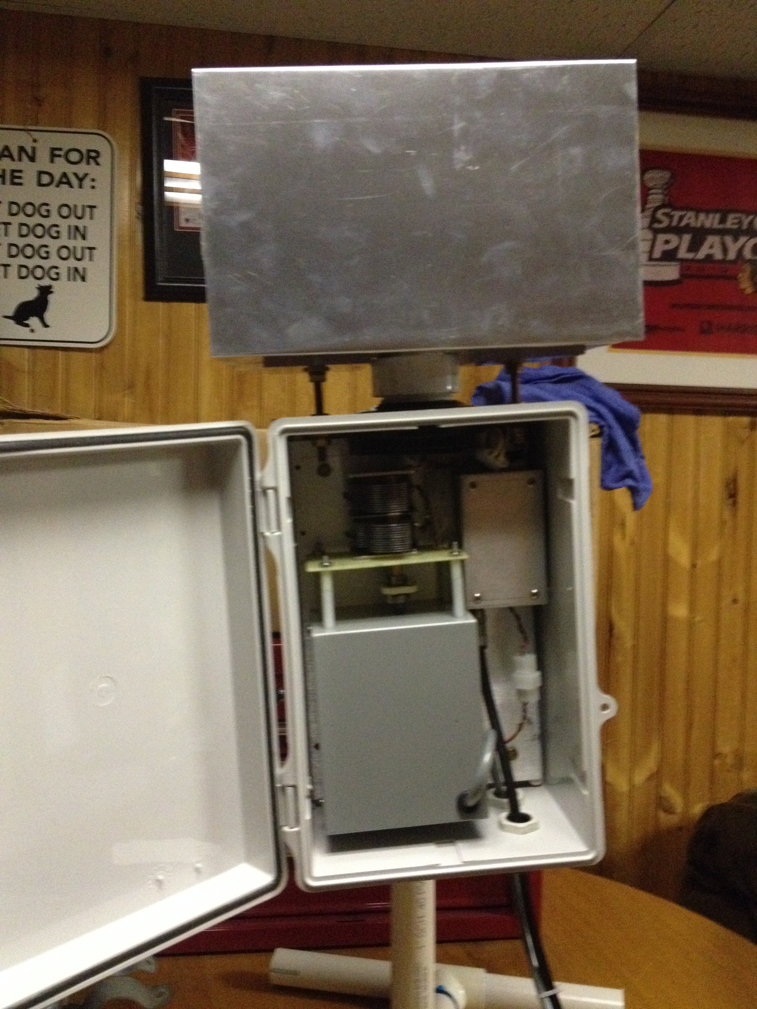
Well, that is an overview of what is going on here. This post will be followed up by at least 3 more posts. The first will discuss some of the technology in the Ferrite Rod RL (the wound rod, the capacitor, and the amplifier) and its tuning mechanism. That is pictured below in a weatherproof enclosure.  The rod per se is not visible, but is located within the aluminum shield above the enclosure.

IMG_0530

The second will discuss the Client app to a greater degree, and a screencap of a typical presentation (along with the typical SDR Console window) is:

Screen Shot

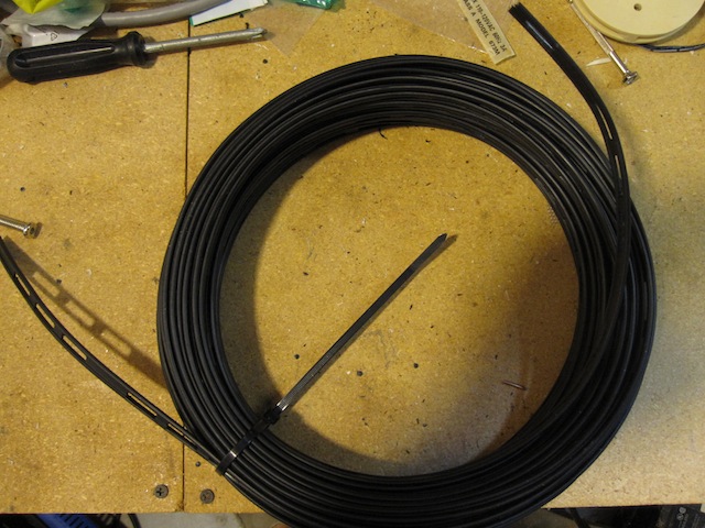
The third will most likely discuss interfacing strategies, as this loop is sited a fur piece from the house, and requires and RF coax, power cabling, and also some form of digital network over which the client and server communicate

I am getting lazy in my old age, but we will most likely throw up a post detailing Rack Shack Rotator modification (converting from the ghastly and slow synchronous motor to a PM DC gearmotor, adding a position feedback pot, and a simple closed loop controller based on an Arduino Pro Mini controller which may be hosted by the Loop Server).

Additionally, the Scenario Visualization tool will most likely merit its own post. This has been one of the funnest parts of this project, and I foresee this tool being a great aid this next season.
Visualization

There is also a long laundry lists of enhancements on the back burner, and we might get around to posting some of these ideas in the future.

Further on down the line we can post some results with regards to performance; there is a lot to evaluate.

This has been – and continues to be – a ton of fun, and also hard work. This antenna represents “where I always wanted to be” with regards to Resonant Loop antennas. This is a big step up from what I used last season, and there is still enormous potential, and lots of new functionality to imagine and implement.

If only the freakin’ thing works…

Yet Another Loop Post

I have been very happy with the Resonant Loop which I have been using for the last couple of years; it has served me well, and will undoubtedly continue to do so in the future. It’s time to move forward, and push it’s capabilities a bit further. My current loop has a loaded Q of approximately 250 at 6925 kHz, and this results in a 3 dB bandwidth of around 28 kHz. This allows the tuning to be rather forgiving at the expense of being absolutely incapable of doing any significant frequency discrimination right within the antenna. To do so will require a loop with a higher Q, a significantly higher Q, and that will not happen using the technology of my current loop.

The loaded Q of a Resonant Loop is primarily determined by 3 things:
– The Q of the winding inductance. To get to the Q levels required, the best practical solution would be to wind the coil with a relatively large copper tubing; stranded wire is no longer practical here.
– The Q of the tuning capacitor. While the tuning diodes used in my current loop really make life easy, they just will not have enough Q at frequencies in the funny band. A high quality mechanical variable capacitor (or vacuum variable capacitor) will be required.
– The impedance presented by the buffer amplifier must be increased. The easiest way to do this is by using the loop windings as an impedance transformer to raise the effective input impedance of the amplifier.

After a lot of number crunching and simulations, I built the following prototype:

IMG_0408

This is shown in a “testing position”, and a mast mount has not yet been built. A quick description of the loop follows.

The loop winding was built from 1/2″ OD soft copper refrigeration tubing, and was designed so that it could be fabricated from a 20′ length of tubing which is commonly available in DIY stores. The preliminary loop inductance is around 11 uH, and at 7000 kHz this winding should exhibit a Q of around 3000. The mean diameter is around 11.5″, and there are 6 turns with a 1″ spacing between turns. Note that copper sweat and brass compression fittings are used to create a solid loop mount to a bar of UHMW; these fittings are mechanical only, and are not part of the electrical circuit.

The capacitor used here is a purchase from Fair Radio Sales a number of years ago, and was a pull from a military ATU. As variable caps go, this is almost as good as it gets. The cap features solid brass construction, and is silver plated in entirety. All insulation is ceramic, and all plate joints appear to be silver soldered. The cap has a built-in 100:1 worm gear reducer with anti-backlash gearing. The measured capacitance range is 15-250 pF.

The windings and capacitor are connected by cobbled up flexible tubular pipes fabricated from some coax cable jacket over which was wound some 0.010″ pure silver foil which was held in place by heat shrink tubing. These pipes are soldered to the capacitor stator and rotor lugs. At the winding end, they are currently clamped onto the copper tubing with SS hose clamps (the clamping area was first silver plated with Cool Amp silver plating powder). At some point, these will be soldered.

Currently, the capacitor is remotely tuned by a PM DC gearmotor via a coupling made from a short length of PVC tubing and cable ties. The power supply is 3 D cells lined up in series against my logbook; I just touch the wire ends to the battery terminals and try to remember which way tunes up and which way tunes down? I have another deck built using an identical variable capacitor coupled to a 100 step/revolution stepping motor which will be used when the control circuits are built.

The white PVC tube above the chassis contains the loop buffer amp. This is just the standard JFET cascode amp used in most of my loops with the exception that the tuning diodes have been removed. A close-up of the hookup:

IMG_0411

The loop tubing was drilled in 3 places to accept the barrels of male 1/4″ quick-connects, and these joints were then soldered. The loop amplifier is connected to these lugs. Note that this connection forms a 3:1 voltage transformer to the amp which results in a 9:1 amplifier input impedance transformation. The approximately 1 Meg amplifier input resistance now appears as a 9 Meg load on the capacitor-winding tank circuit which helps to keep the loaded Q high.

In starting this project, there were some known knowns. Primarily, I was pretty confident that a loop winding could be fabricated which would give me the proper inductance while at the same time giving me a required Q of around 3000. This build has proven that to me. There was also a major unknown known. It is extremely difficult to find hard data on the real Q of a mechanical variable capacitor of this type. The tubes are littered with vague statements which describe the Q of such caps as “very high”, “excellent”, and so forth. There are a couple of sites which have detailed Q information on a particular cap (which looked promising to me). But not this cap. Having built this loop, back calculations seem to suggest that the Q of this cap is somewhere around 1200-1500 at 6925 kHz, and this figure seems realistic to me.

My goal in this build was to raise the Q of a receiving loop by a factor of 2 or 3 from its current value of 250; I would be happy for a Q of 600. This would give an 3 dB BW of around 12 kHz at 6925; good, but not good enough to pry a pesc off of a pirate’s signal. So, what did we get?

To be honest, these results are preliminary, and vary all over the place. This is to be expected for such high Q circuits. The measurements can be tricky, and the results can be skewed by environmental things such as humidity, proximity to other objects, etc. At this point, Q measurements are consistently falling into a range between around 600 and 1050. I most commonly see values around 850 at 6925 kHz, and this thrills me to no end. A Q of 850 implies a 3 dB BW of around 8 kHz at 6925; if you squint, you can imagine that with a little more Q, some serious frequency discrimination can be accomplished.

How much more Q? I would LOVE to have a loop which exhibits a real 3 dB BW of 6 kHz at 6925; this would require a loaded loop Q of around 1150. At this point it is beginning to look realistic to me.

How do you get there with the current build configuration? One can calculate that at the current operating point (6925 kHz, Q = 850) that the LC tank circuit has a total effective series resistance of around 0.57 Ohms. I have gotten the greatest Q gains in the prototype by monkeying with the 2 connections between the winding and the capacitor, and I think that there is room for improvement there. Every milliohm counts. This particular capacitor also has the same Achilles heel that many variable caps have. the connection to the rotor. In this cap, there are 2 silver buttons on a spring loaded leaf, and these buttons wipe a silver commutation ring on the cap rotor. I have yet to do a really thorough cleaning of the sulphide layer on the ring, and have left this trump card in the back pocket. When I can no longer push the Q any higher, we will look here. There is also the possibility that this wiping contact can be replaced by a flexible silver tape, soldered to the ring.

There is a backup plan. This loop was built rigidly so that it would run in a stable manner at its tuned operating point. This would be a requirement for the next step, which would be to upgrade the loop to a so-called “regenerative loop” which could possibly supply some additional Q. More about this later.

In the few nights that I have used this for DXing, I have started to become familiar with the listening characteristics of this loop as compared to my standard loop. Although my current Neanderthal tuning supply makes it hard to peak the loop on a signal, the response peaks as seen on an SDR FFT plot are much more pronounced at Q=850 than they are at Q=250. With a 100 kHz view span, the 250 loop gives you a pretty good heads up look at a wide chunk of frequency spectrum; it’s hard to miss a weak signal off to the side of the loop response peak. Not so with the 850 loop; signals off to the side may be attenuated deeply, and it is quite possible to miss stuff.

On strong signal reception (say >= S7) it appears to be a coin toss between the 2 loops; both perform adequately. On weaker signals, I am giving the preliminary edge to the 850 loop. The 850 loop appears to be giving me better S/N ratio on weak signals, but I will hold this call until we are deeper into the season and storm noise lessens.

Which brings up another observation: when I had a wire antenna up, I noted that storm QRN as heard via the 250 loop was a lot “softer” than the crashes heard via a wire antenna. In the headphones, the storm noise was still there, but it tended to be less harsh and grating on the ears, and it was easier to “hear through” the noise on the 250 loop. I am noting now that storm QRN heard via the 850 loop is even mellower than that heard through the 250 loop. There is something going on there, as there is even a difference in lightning strike rendering in the SDR waterfall.

Well, enough for now.

Automating Loop Design

Spring is here finally (tra-la! tra-la!) and it’s time to get back into the yard to repair Winter’s damage and install new antennas. In particular, I want to possibly upgrade the Resonant Loop I am using for 90% of my DX time. In the past, this has generally involved intensive and error-prone hand calculations, and I was looking for a way to automate the process, or at least portions of the process. Thus, I wrote a bit of code to help streamline the design and evaluation, and hopefully help to root out the best solution.

The loops I use are usually square loops built on PVC pipe frames. These loops will almost always have a pair of identical windings separated by a center gap; this gap dramatically reduces the winding parasitic capacitance an helps to extend the tuning range. The code I wrote assumes a center gap of 3″ (which is typical for construction on 3/4″ PVC pipe) and a winding pitch (gap between adjacent turns) of 1/2″, but these values may be easily changed for exploration into other design areas.

One of the more difficult problems is computing the loop inductance as a function of the number of turns and loop side length, so the first part of the code does this for me. The code generates an array of inductance values which represents the computed inductance for a loop with turns counts of 2, 4, 6, 8, 10, and 12 turns, and side lengths of 0.25 – 1.125 meters, and then displays the results graphically. These curves may be of use to anyone who is contemplating building a loop.

Inductance Curves

The curve rendered in red represents a side length of 0.25M, and the black curve represents 1.125M. These curves represent the solution array of inductance values. One of these values might be appropriate for my loop design, but which one? To select an appropriate inductance value, the code needs to know about the intended loop tuning range, and also the capacitor used to tune the loop. From that info, it can compute the winding inductance which is required.
If you scan horizontally along any horizontal grid line (along any given value of inductance) you will note that there are several turns-side length value pairs which could generate that inductance. The question becomes: “Which is the best or most appropriate for the design goal?” Which begs the question “What is the design goal?”. Resonant loop design is the art of compromising performance in one area against several other areas. In this code, the design goal is kept simple: from the turns-side length pairs which generate the proper inductance ( +/- 20% ) we are going to select the solution which has the greatest product of turns and loop area; we are selecting for maximum Numerical Aperture.

The code then iterates through the array of inductance values, and determines if a value meets the inductance requirement dictated by our desired tuning range. If it finds a solution, it computes the Numerical Aperture ( number of turns times the side length squared), and tracks the solution which represents the maximum Numerical Aperture. When done, it presents the best solution in a dialog box, or…

Dialog

The code is telling me that I should make a loop which has 2 turns, with a side length of 44″, which is a point along the red curve in the graph. This is interesting, since my current loop uses 4 turns with a side length of 20″, which is point along the Ch. 2 curve in the graph. Whatever. Knowing the number of turns and side length, the code finishes off by generating a graph of important loop parameters over the loop tuning range. These are:
– The loop Tuning Curve (capacitance vs. frequency)
– Effective Height He – the length of a vertical wire having the same output as this loop
– Figure of Merit with respect to Pattern (FOMP) – the ability of the loop to generate a pattern null

Params Curve

And that’s about it. If you are interested in the code used to generate these graphs, you can see that here:

https://www.mediafire.com/?uvkbx5l6o6tyc85

This contains greater comment detail than is presented here.

Time to Call the Service Guy

After a rather moderate summer, Chicago has seen the appearance of a couple of spells of nasty heat and humidity. Along with this I have noted the appearance of a new noise in the 43 meter band and elsewhere. It is typically noted at around an S5 level with my resonant loop spun to the preferred azimuth. It begins in the late afternoon, chugs away at a rather high duty cycle for a couple of hours, and then settles in to a low duty cycle operation (a few minutes every hour) by 0100z. It has every indication that it is mains-related, and did not correlate with anything in my house. In the past I have had problems with leaky or grunged insulators on utility power poles, and the noise resulting from that has always exhibited a more random and intermittent nature; it has also tended to exhibit strengths in the range of S9 to S9+5. This new noise was kinder and gentler, but would still interfere with my ability to note weak carriers in the SDR waterfall. When I come down to the shack after work, I like to see an S2 noise floor in the late afternoon, when storm noise is not audible, with my preferred SDR gain settings ( IF = +18dB, RF = -10dB ). This was not the case.

I have just recently installed a rotor on the loop, a HyGain AR-303 light duty rotator which can easily handle a loop of this size. The goal then was to see what could be done about dealing with and possibly identifying the source of) this noise.

A small loop exhibits a “Figure 8″ reception pattern; there are two lobes of maximum reception which are aligned with the plane of the loop. There are 2 reception “nulls” which are at right angles to the plane of the loop. In theory, these nulls could be pointed at an offending noise source to minimize its impact on reception. The “Standard Loop” described in the HFU post here http://www.hfunderground.com/board/index.php/topic,12084.0.html has been designed to offer a good balance of reception properties. While I have slanted the design towards sensitivity, there is still enough ability to depress local noise sources. Let’s see how much.

Maximizing the noise by loop rotation, this is what was seen on the SDR waterfall:

AC Noise

The brightening of the waterfall palette is clearly seen across the resonant bandwidth of the loop, and it is easy to see that weak carriers or signals about 6925 (or at any frequency in the SDR display range) would be obscured. The SDR is reporting an average signal strength of S5 at 6925. To be honest, this would not be an issue if everyone was heard at S9+10; there might be some background buzzing in the audio. But for DX, I could not live with this.

The loop was then rotated so that the noise was minimized, and another screen cap was taken. The waterfall now appeared like this:

No Noise

The noise about 6925 has been reduced significantly, and the SDR is now reporting a signal strength of S3 at 6925. This is a bit higher than what I would like, but I can live with that. Using a light touch on the SDR noise blanker helps to clean up most of the remaining audio buzz without introducing distortion.

Note also that a couple of things which were not visible in the previous image are now visible. The spur which we commonly see on 6970 is now there, as is a big blob of noise just above 6980. I do not know what this is, but I see it all the time. It generally hangs out around 6980 plus multiples of about 105 kHz above and below 6980. It generally stays close to this frequency, but it may move up or down and appear as massive interference at 6925. But it can be suppressed also. If you compare the previous image (max noise) and with this it can be seen that these two noise sources are at about 90 degrees apart in azimuth.

A better way to look at this would be by looking at the SDR waterfall as the loop is scanned. In a separate session (the following day) I again looked at these two noise sources by scanning the loop through approximately 180 degrees (from rotor north to rotor south) and taking took a screen cap of the entire scan. That is here:

Loop Scan 29Aug13

This image clearly shows that around the time the rotor was pointing due east (lobes of max reception pointing east and west, nulls pointing north and south), the noise was minimized, It also shows that the rough azimuth of the second noise source around 6980 could be determined from the rotor position. The lobes of the null are not sharp, and there is a spread of a few degrees where the noise is minimized as a consequence of the loop null pattern. The loop is dealing with the noise fairly effectively. It seems to indicate that a noise reduction of about 2 S Units (12dB) is being observed.

A more accurate way to measure the noise reduction was tried. I use SDR Console to support the SDR-IQ, and the most valuable tool this software has is a Strength History window. I set the Strength History range to 60 seconds, and again scanned the loop from rotor north to south, while the history window recorded the loop output in dBm. Here is what I saw:

Loop Scan 28Aug13

I currently have no way to calibrate the scan; I don’t know exactly when the scan started or stopped in the strength chart, but a rough guess would be that it started around 40 seconds into the chart, and ended around 10 seconds. No matter; the pattern minima and maxima are easy to see, and these are approximately -110 and -94dBm, a difference of 16dBm (approximately 2.6 S Units).

This is a typical value of the suppression which can be obtained against a local noise source. I have seen suppression against particular noise sources of up to 24dB (4 S Units), but this seems to be about the limit. I no longer freak when noise pops up; loop rotation can generally solve most of the problem, and judicious use of the software noise blanker generally cleans up the rest. As long as there is a reasonably wide azimuthal difference between the noise source and the desired station, effective noise reduction can be accomplished.

This was all done using an unshielded resonant loop; at some point in the future I would also like to try this with a Wellbrook loop.

It’s been a long boat ride here, but the noise source was pretty easy to ID by sighting through the loop. When the noise was suppressed, the null pointed directly at my neighbor’s air conditioning unit, and it looks to me like it’s time for him to call his service guy. I would be absolutely willing to do a quick and cheap fix for him with my Sawzall…

A Sloped Folded Dipole Antenna for 43 Meter Band

While I’ve had very good reception using my sky loop antenna, I wanted something that would have better low angle radiation sensitivity, for improved reception of distant stations.

The sky loop is 670 ft in perimeter, and runs around the yard at a height varying between about 20 and 50 feet, depending on how tall the trees are. In order to get a better low angle radiation pattern, an antenna, for the 43 meter band anyway, should be higher. I don’t have two tall trees suitable spaced for erecting a standard dipole high enough for 43 meters. I do have one tall tree however, so I decided to consider a sloped dipole.

Below is the NEC simulation of a such a dipole:

The low angle radiation sensitivity is indeed pretty good, and there is some directionality as well.

I decided to go with a folded dipole, as my previous experience with them has been good, they seem to share the common characteristic of all loop type antennas of not picking up a lot of local noise and RFI.

A folded dipole is constructed using two conductor cable, such as TV twin lead or ladder line. I went with the latter as twin lead is not very rugged:

As the feedpoint impedance of a folded dipole is about 300 ohms, a balun should be used. In this case I used a 4:1 balun, which then feeds 75 ohm RG-6 coax:

I used some short sections of plastic conduit for the end and center supports, to provide some mechanical rigidity:

The standard dipole formula was used, resulting in a length of 67 feet. The two far ends of the ladder line have their insulation removed and the two wires are shorted together.

At the center of the antenna, one of the conductors is cut, and the balun is attached here, as shown below:

I used nylon wire ties to secure everything.

Here is the completed antenna, the two sections of ladder line are temporarily spooled to keep them tidy until the antenna is erected:

The high end of the antenna is at about 55 feet. the low end about 15 feet. A rope is attached to the balun eye hook and goes over another tree, providing a little more mechanical support.

For normal daytime reception, it works about the same as the sky loop on 43 meters. At this time of the day, propagation is NVIS, and the signal comes down at a high angle. I was not expecting much of an improvement here.

Later in the day, results have been quite good, as I hoped. Late in the afternoon, I decided to try 6160 CKZN from St Johns, Newfoundland. With the sky loop, I barely had a carrier, while with the folded dipole, I had audio.

All in all I am quite pleased with the performance, and am switching to using this antenna for my overnight recordings on 43 meters.